Trial Design Options • ofpetrial

The ofpetrial package offers various trial design types. This vignette provides examples of availabl design types. Let’s first prepare experiment plots to which we assign rates using various trial design options.

library(ofpetrial)

n_plot_info <-
  prep_plot(
    input_name = "NH3",
    unit_system = "imperial",
    machine_width = 30,
    section_num = 1,
    harvester_width = 20,
    headland_length = 30,
    side_length = 60
  )

exp_data <-
  make_exp_plots(
    input_plot_info = n_plot_info,
    boundary_data = system.file("extdata", "boundary-simple1.shp", package = "ofpetrial"),
    abline_data = system.file("extdata", "ab-line-simple1.shp", package = "ofpetrial"),
    abline_type = "free"
  )

viz(exp_data, type = "layout")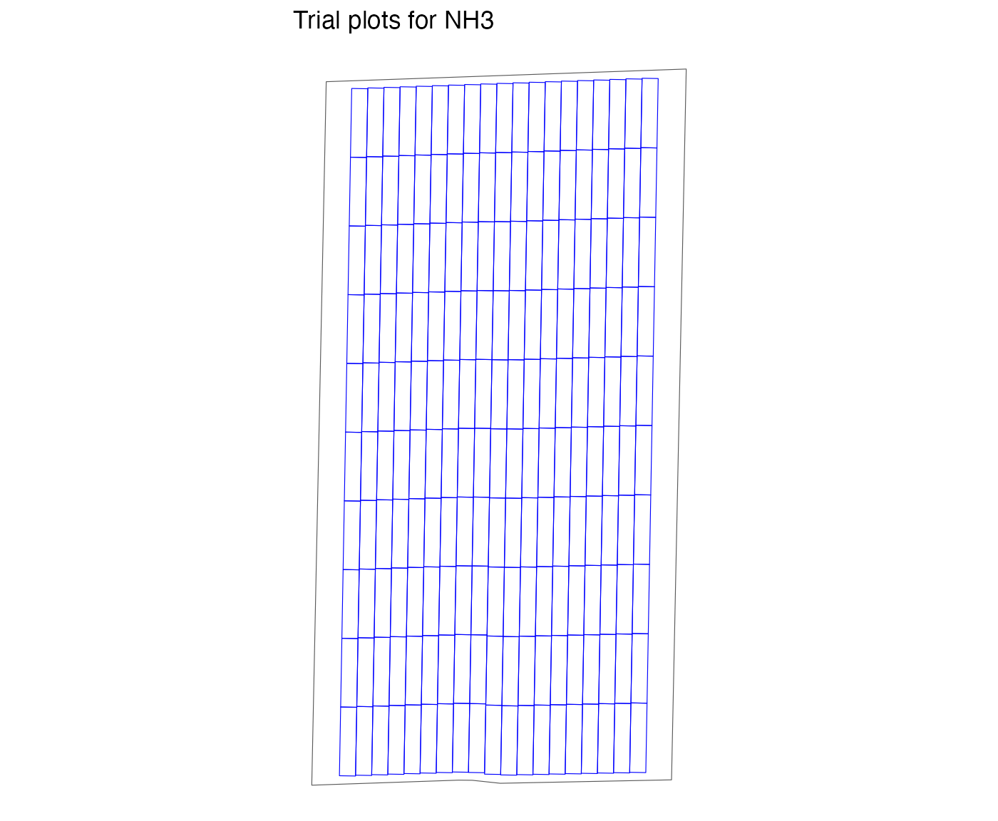

We will be assigning rates to the experimental plots using various trial design types below.

Latin Square (“ls”)

By default, here is what design_type = "ls" produces.

n_rate_info <-
  prep_rate(
    plot_info = n_plot_info,
    gc_rate = 180,
    unit = "lb",
    rates = c(100, 140, 180, 220, 260),
    design_type = "ls"
  )

td_ls_d <-
  assign_rates(
    exp_data = exp_data,
    rate_info = n_rate_info
  )

viz(td_ls_d)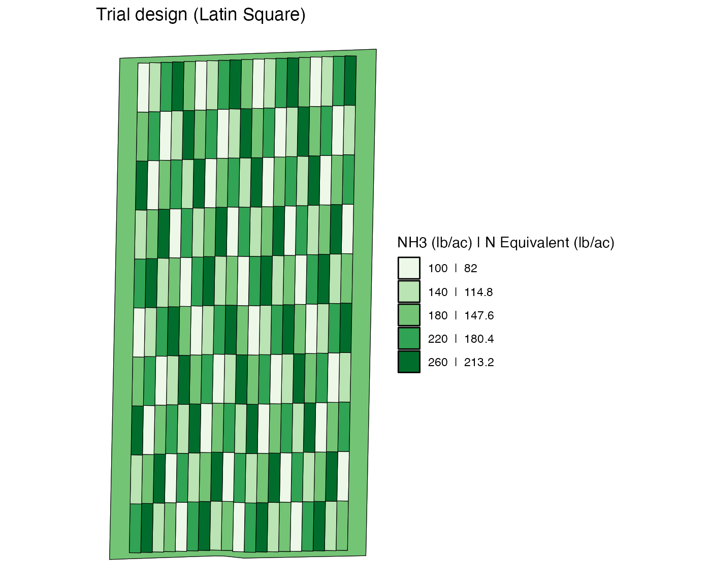

Note that the trial design produced by assign_rates() is randomly picked from a pool of candidate Latin Square designs. If you would like to reproduce the same trial design later, you can use set.seed().

set.seed(89934)

td_ls_d <-
  assign_rates(
    exp_data = exp_data,
    rate_info = n_rate_info
  )

viz(td_ls_d)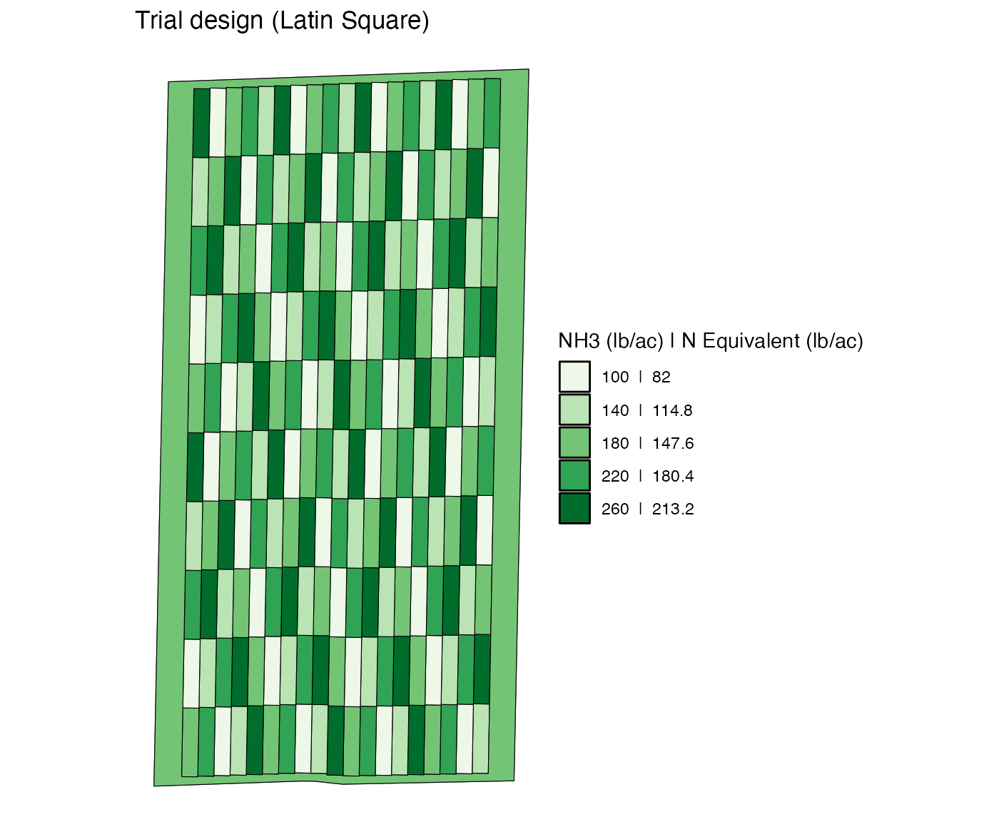

However, you can customize the spatial pattern of input rate when design_type = "ls" using the rank_seq_ws and rank_seq_as options. To do so, it is important to understand how plot_id and strip_id are assigned to each of the plots. Here are their maps.

ggpubr::ggarrange(
  viz(td_ls_d, type = "strip_id"),
  viz(td_ls_d, type = "plot_id"),
  ncol = 2
)

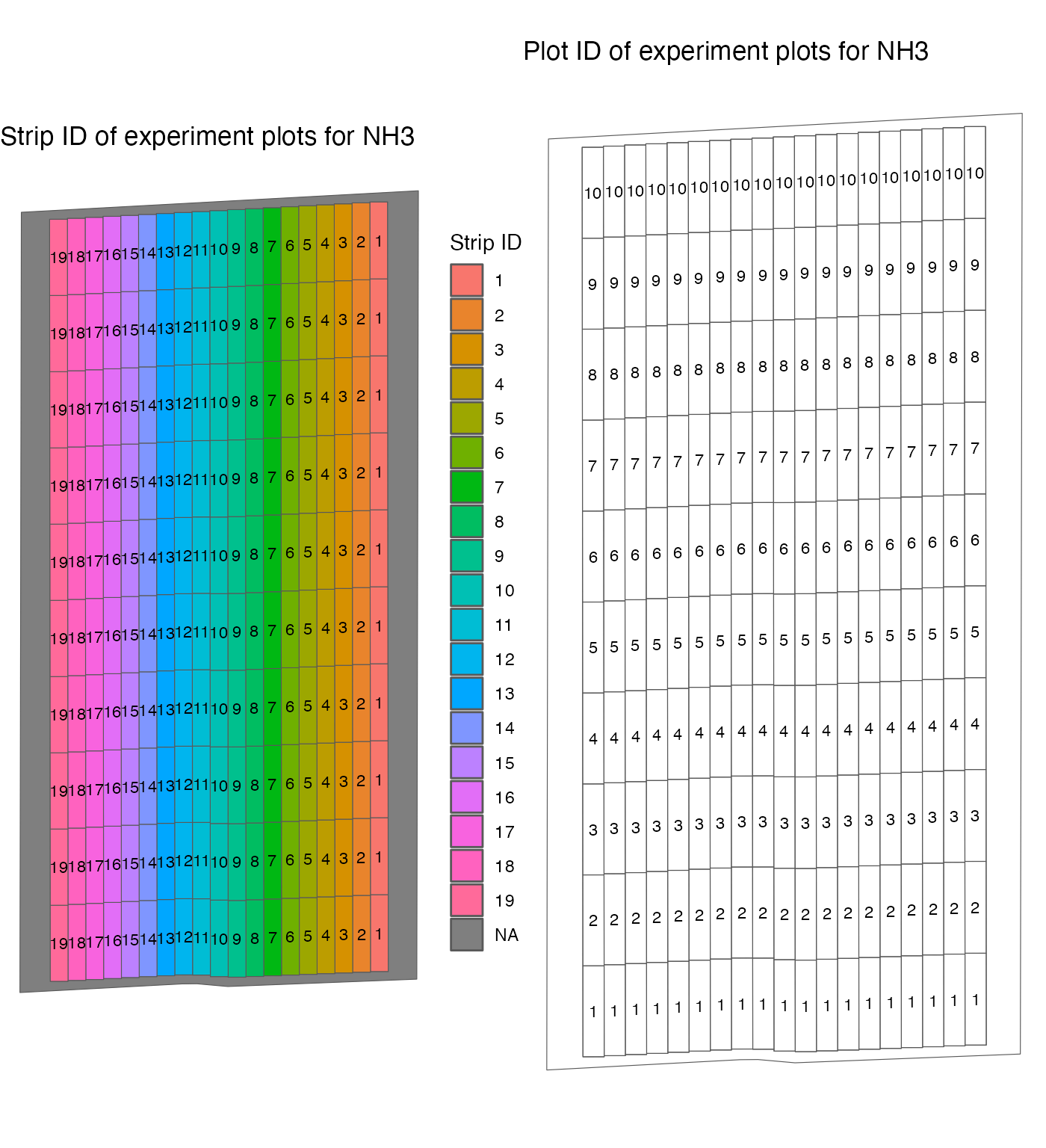
As you can see, plot_id is the unique numeric identifier assigned to each of the plots within a strip. So, there are multiple plots with the same plot_id values, but a combination of strip_id and plot_id uniquely identifies a plot.

The rank_seq_ws option specifies the order of rate rankings to be repetead within a strip (this is why _ws at the end of the function). Suppose you have rank_seq_ws = c(5, 4, 3, 2, 1). 5 refers to the 5th-ranked (highest) rate, which is 260 because we have rates = c(100, 140, 180, 220, 260) above. 1 refers to the first-ranked (lowest) rate, which is 100. Rates are assigned in this order to the plots within a strip. The rank_seq_as option specifies the order of the rate rankings of the very first plot of each strip across all the strips. So, for example, if rank_seq_as = c(1, 4, 3, 2, 5), then the first plot (plot_id == 1) of the first strip (strip_id == 1) will be assigned rate rank of 1. The first plot of 5th strip (strip_id == 5) will be assigned rate rank of 5. This sequence will be repeated until the first plot of all the strips are assigned a rate rank. Now, for a given strip, rate ranks specified by rank_seq_ws will be repeated starting from the rate rank of the first plot. For example, the first plot of the 3rd strip has a rate rank of 3 (so, 180). This means that the code will go over the rest of the rate ranks in rank_seq_ws (2 and 1), and then go back to the beginning of rank_seq_ws, which is 5. So, for the third strip, the rate rank of its plots look like this.

rank_seq_ws <- c(5, 4, 3, 2, 1)

data.frame(
  plot_id = 1:10,
  rate_rank = c(3, 2, 1, rank_seq_ws, rank_seq_ws[1:2])
)
#>    plot_id rate_rank
#> 1        1         3
#> 2        2         2
#> 3        3         1
#> 4        4         5
#> 5        5         4
#> 6        6         3
#> 7        7         2
#> 8        8         1
#> 9        9         5
#> 10      10         4

Let’s try few examples.

n_rate_info$rank_seq_ws <- list(c(1, 2, 3, 4, 5))
n_rate_info$rank_seq_as <- list(c(1, 2, 3, 4, 5))

td_ls_1 <-
  assign_rates(
    exp_data = exp_data,
    rate_info = n_rate_info
  )

viz(td_ls_1, type = "rates")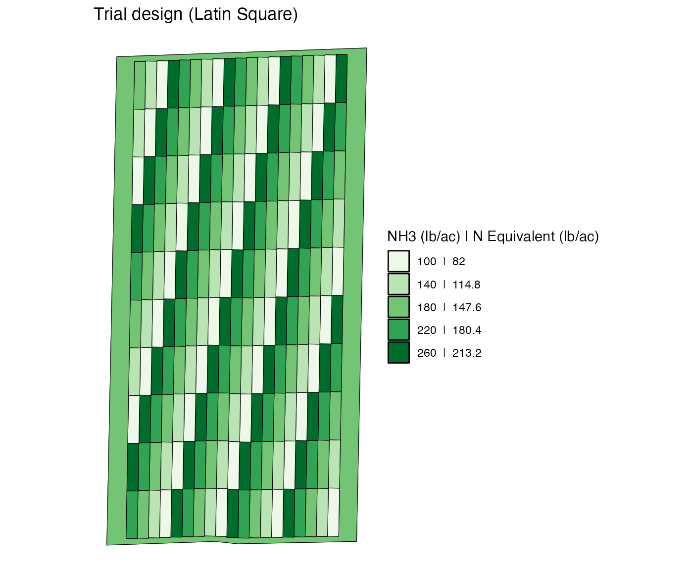

n_rate_info$rank_seq_ws <- list(c(5, 2, 4, 1, 3))
n_rate_info$rank_seq_as <- list(c(1, 5, 2, 4, 3))

td_ls_2 <-
  assign_rates(
    exp_data = exp_data,
    rate_info = n_rate_info
  )

viz(td_ls_2, type = "rates")

Strip trial (“str”)

You can design a strip trial using design_type = "str". By default, it repeates a sequence of rates like below.

n_rate_info <-
  prep_rate(
    plot_info = n_plot_info,
    gc_rate = 180,
    unit = "lb",
    rates = c(100, 160, 220, 280),
    design_type = "str",
  )

td_strip <-
  assign_rates(
    exp_data = exp_data,
    rate_info = n_rate_info
  )

viz(td_strip, type = "rates")

Just like the “ls” option, you can specify the spatial pattern of strip rates using the rank_seq_as option. The code below repeats 100 (rank 1), 280 (rank 4), 220 (rank 3), and 160 (rank 2). Since the strip trial has a single rate per strip, rank_seq_ws is not available unlike design_type = "ls".

n_rate_info <-
  prep_rate(
    plot_info = n_plot_info,
    gc_rate = 180,
    unit = "lb",
    rates = c(100, 160, 220, 280),
    rank_seq_as = c(1, 4, 3, 2),
    design_type = "str",
  )

td_strip <-
  assign_rates(
    exp_data = exp_data,
    rate_info = n_rate_info
  )

viz(td_strip, type = "rates")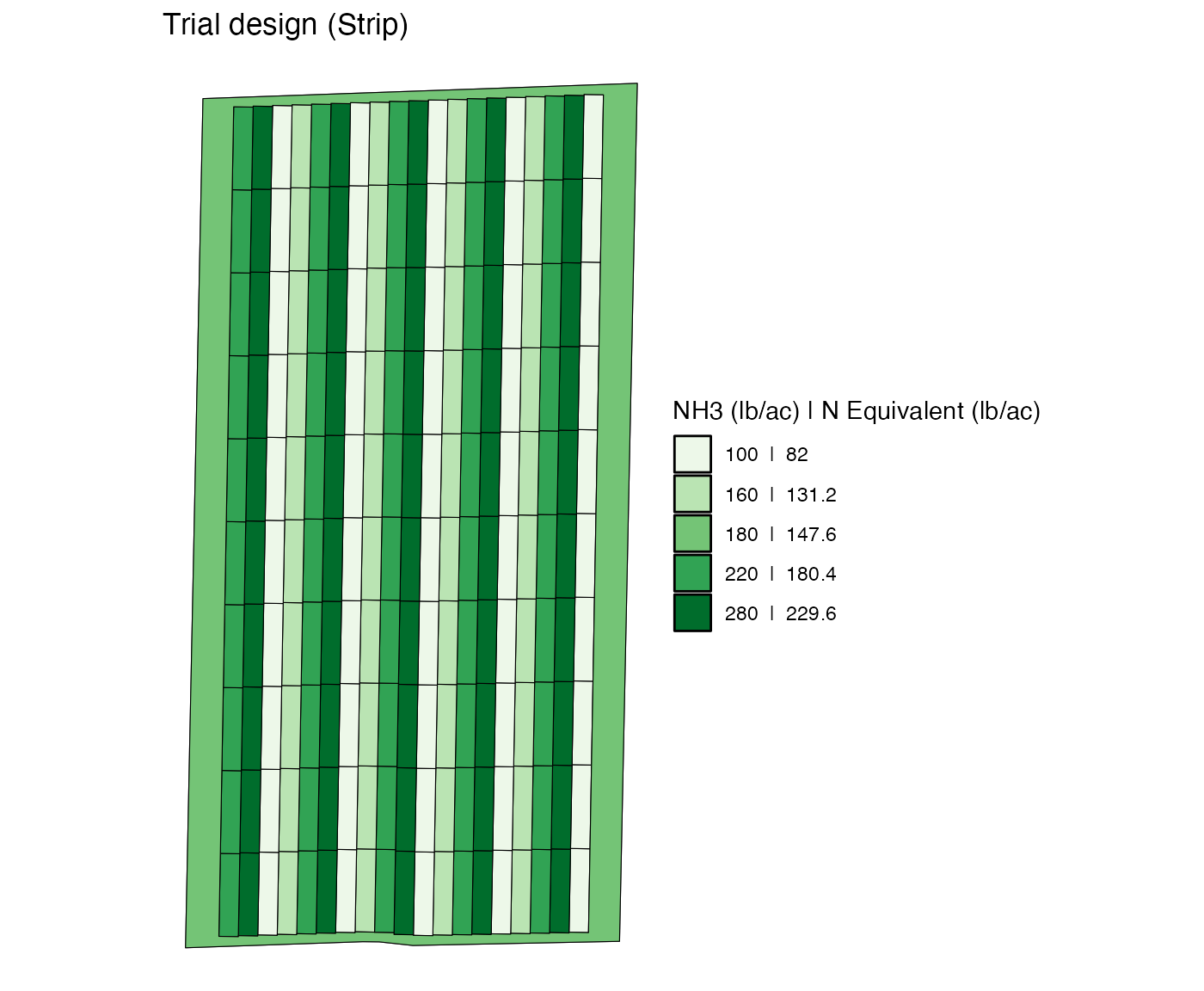

For the strip trial, you can specify the full sequence unlike the other design options. We have a total of 19 strips in this experiment.

#--- total number of strips ---#
max(exp_data$exp_plots[[1]]$strip_id)
#> [1] 19

Let’s provide a vector of length 19 to rank_seq_as.

n_rate_info$rank_seq_as <- list(c(1, 4, 3, 2, 2, 3, 4, 1, 3, 2, 1, 4, 2, 3, 1, 4, 4, 2, 3))

td_strip <-
  assign_rates(
    exp_data = exp_data,
    rate_info = n_rate_info
  )

viz(td_strip, type = "rates")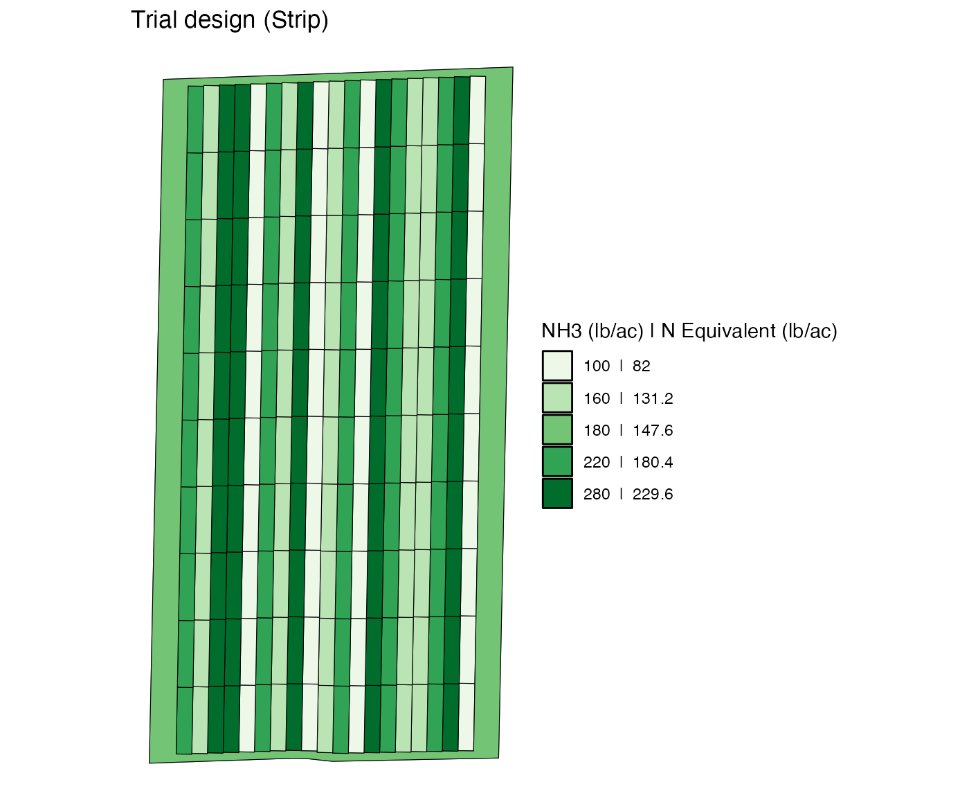

Randomized Strip (“rstr”)

You can create a randomized strip design using the “rstr” option as follows.

set.seed(329544)

n_rate_info <-
  prep_rate(
    plot_info = n_plot_info,
    gc_rate = 180,
    unit = "lb",
    rates = c(100, 160, 220, 280),
    design_type = "rstr",
  )

td_randomized_strip <-
  assign_rates(
    exp_data = exp_data,
    rate_info = n_rate_info
  )

viz(td_randomized_strip, type = "rates")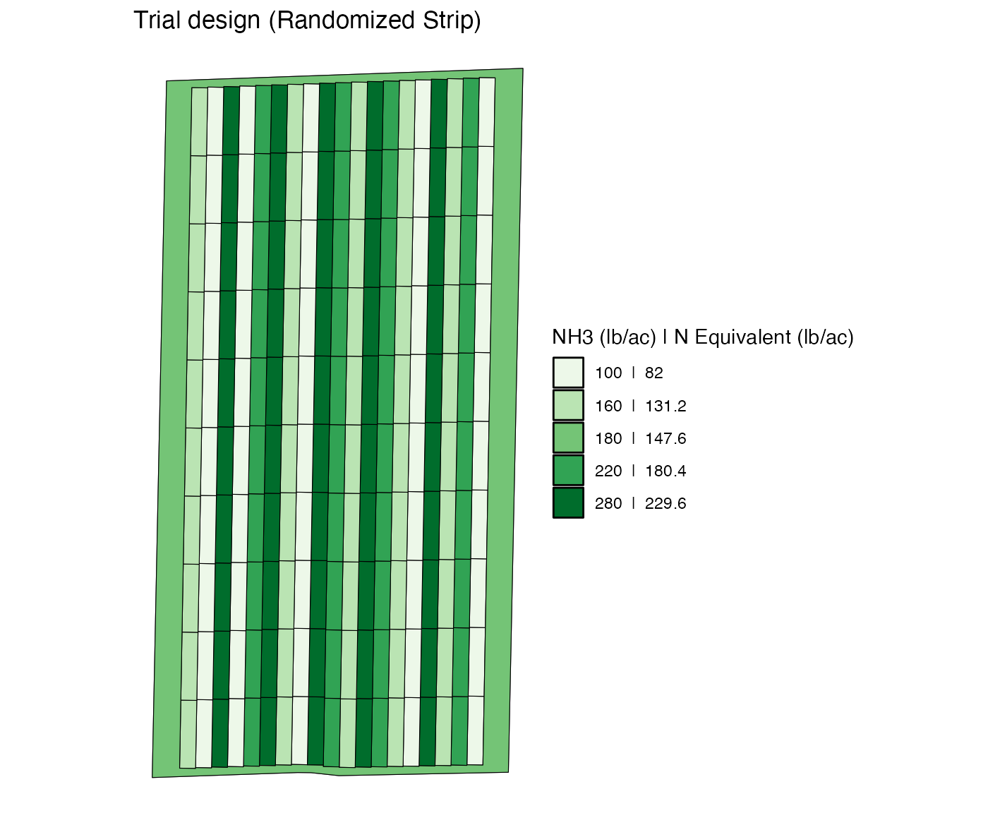

This design is not completely randomized. Rather it is randomized inside a block of strips. Here, a block consists of four consecutive strips because four distinct rates were provided by the user.

Randomized Block (“rb”)

You can crete a randomized block design using the "rb" option.

n_rate_info <-
  prep_rate(
    plot_info = n_plot_info,
    gc_rate = 180,
    unit = "lb",
    rates = c(100, 140, 180, 220, 260),
    design_type = "rb",
  )

td_rb <-
  assign_rates(
    exp_data = exp_data,
    rate_info = n_rate_info
  )

viz(td_rb, type = "rates")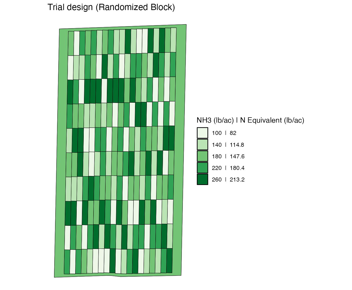

When design_type = "rb", blocks are created internally when assign_rates() is run. Here is what blocks look like.

add_blocks(td_rb) %>% viz(type = "block_id")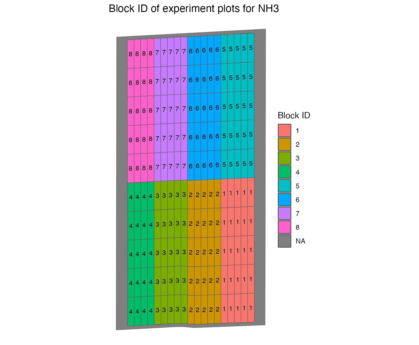

Since there are five distinctive rates, each block consists of five by five plots. In each of the block, the five rates are randomly assigned in a way that each of the rates appear exactly five times.

Extra Jump-conscious Alternate (“ejca”)

This design alternate high-rate strip and low-rate strip, thus avoiding sudden changes in input rates so that machines can handle them. EJCA is more machine friendly than JCLS.

n_rate_info <-
  prep_rate(
    plot_info = n_plot_info,
    gc_rate = 180,
    unit = "lb",
    rates = c(100, 140, 180, 220, 260, 300),
    design_type = "ejca",
  )

td_ejca <-
  assign_rates(
    exp_data = exp_data,
    rate_info = n_rate_info
  )

viz(td_ejca, type = "rates")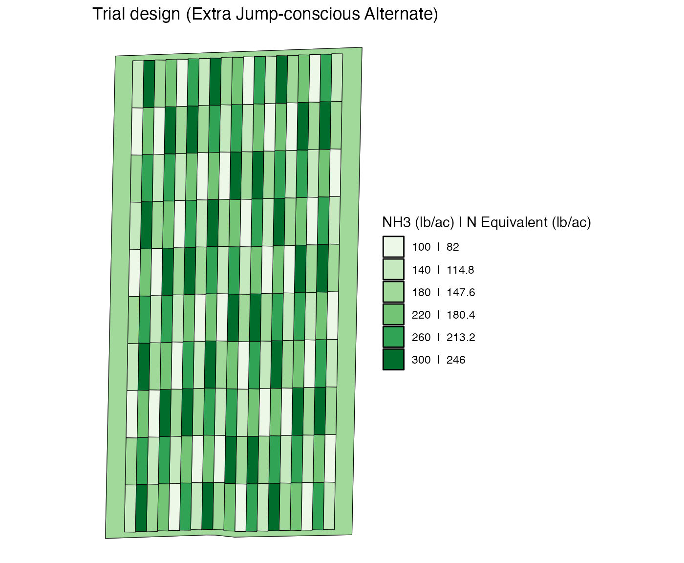

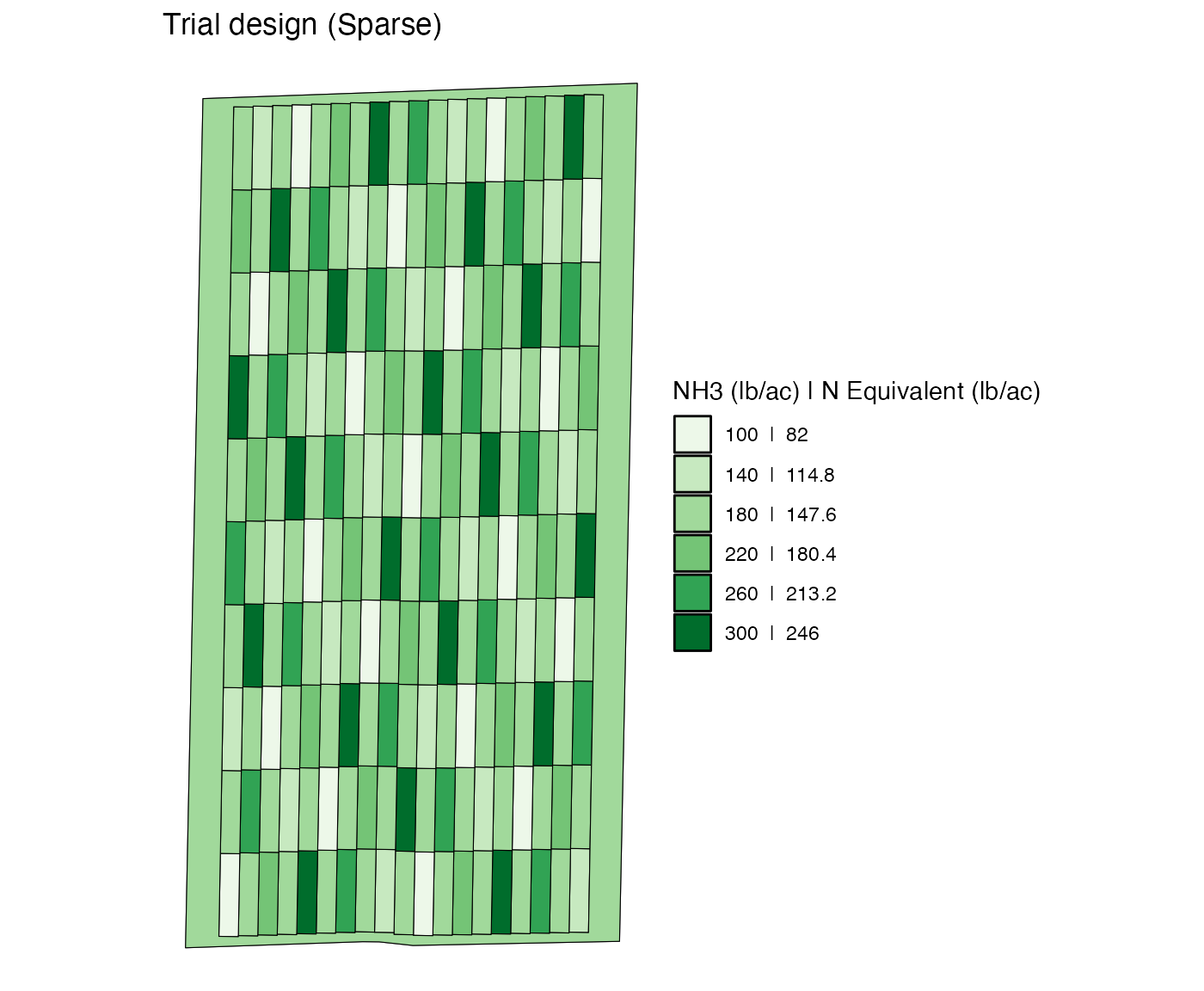
Sparse (“sparse”)

Sparse design with the "sparse" option generate a trial design so that every other experimental plot has the status-quo rate (business-as-usual rate). This can potentially alleviate yield loss associated with lower rates compared to other designs as lower rates happen less frequently.

n_rate_info <-
  prep_rate(
    plot_info = n_plot_info,
    gc_rate = 180,
    unit = "lb",
    rates = c(100, 140, 180, 220, 260, 300),
    design_type = "sparse",
  )

td_sparse <-
  assign_rates(
    exp_data = exp_data,
    rate_info = n_rate_info
  )

viz(td_sparse, type = "rates")